Data diagnostics for CSV and Excel before machine learning

This data diagnostics tool examines a CSV or Excel file before you prepare a machine learning model. Choose your task, target and the variables to retain. You receive metrics, charts and recommendations based on the values in the table. Then choose your cleaning rules, check their effects and validate the preparation. You can download cleaned data with the applied rules and your comments, in Excel sheets or separate files for CSV.

Import a table and check how it was read

Choose the right file and sheet

Start with Choose a file or drop your table in the upload area. The diagnostic accepts CSV, TSV and XLSX, up to 15 MiB, 50,000 data rows and 100 columns. Exceeding a limit produces a message; extra observations are not simply removed to obtain a result. A preview of a few rows should therefore not be confused with an analysis limited to those rows.

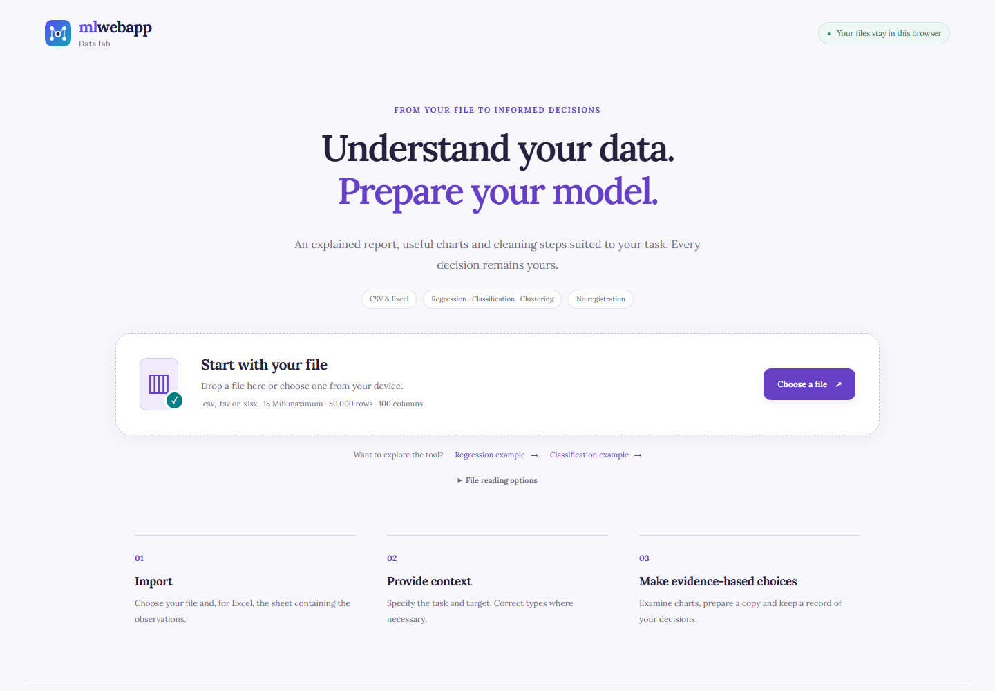
For an Excel workbook, choose the sheet containing the observations. The diagnostic reads one sheet at a time and does not arbitrarily combine tables. Also check the header row: a sheet may begin with a title or description before the column names. After changing sheets or reading options, use Read the file again, then recheck the columns and target.

Each row should represent a clear unit of observation: a person, order, measurement or event. If a workbook contains side-by-side tables, subtotals or comment rows among the observations, first prepare a consistent tabular sheet. The diagnostic can detect some symptoms of an unsuitable structure, but it cannot determine the domain meaning of each row.

Check CSV conventions

A CSV file does not always use a comma as its delimiter. Depending on the export, fields may be separated by semicolons, tabs or pipes. Automatic detection is an initial choice to check in the preview. If everything appears in one column, examine the delimiter before concluding that the data is faulty or deleting that column.

Encoding determines how bytes represent characters. UTF-8 is the default; Windows-1252 is an explicit option for files that use it. Garbled accented characters call for checking the encoding and source file. The diagnostic preserves strings during import: a code such as 00123 is not automatically converted to a number, because its leading zeros may be meaningful.

The field delimiter and decimal separator are different conventions. A CSV may use semicolons between columns and a comma in 12,5. Adjust the decimal convention under Analysis rules where necessary, then update the report. The diagnostic does not silently strip units or thousands separators: 12 kg requires a decision about the format and unit.

Read Excel warnings

This tool does not accept XLS or XLSM. For XLSX, formulas are neither executed nor recalculated. The diagnostic uses results saved in the workbook where available and flags formulas without a saved result. Those saved values may be outdated. If freshness matters, check the workbook in your spreadsheet application before importing it again; do not replace a missing value with zero without justification.

Dates also need a clear convention. The diagnostic recognizes unambiguous ISO representations and handles Excel date cells using the available information. A value such as 01/02/2026 is not enough to choose between two interpretations. Check the column documentation and prepare an explicit format. A duration, Excel serial number and calendar date do not represent the same thing.

Choose the task, target and variables

Define the question to answer

Regression predicts a numeric quantity; classification predicts a category. Choose the task from the question, then select the column to predict, called the target variable. A column containing 0 and 1 may represent two classes. Its numeric appearance does not require a regression task. The diagnostic checks properties of the format, but the meaning of the target still needs to be confirmed from the file’s context.

Exploration mode describes the table before you choose a learning task. Clustering looks for structure among observations without a supervised target. In these modes, the diagnostic does not present assumed ground-truth groups or infer a class count from column names. Choose the variables and review their scales before defining a distance or clustering method.

Names in an imported file do not trigger automatic target selection or column exclusion. A variable called result may serve a different purpose in your project. Changing tasks does not justify reconstructing labels either. The diagnostic preserves supplied values and lets you choose the column that answers your question. Built-in examples, by contrast, open a view already prepared for the stated task.

Exclude or restore any column

Under the target, Variables to exclude lets you select and exclude a column. Repeat for several variables, or use the selection checkboxes in the Columns tab. Undo any exclusion with Restore. The diagnostic then recalculates its scope. This is a general-purpose choice: it works with your own column names and does not depend on the example dataset.

You can also deselect the target. This clears its selection, and the diagnostic requests another target before continuing with supervised preparation. Choosing an excluded column as the target explicitly restores it. The target remains separate from the input features. Check the input count and displayed name before downloading a script, particularly after several changes to tasks or exclusions.

Excluding a column does not destroy it in the original file. It removes the column from the active report, candidate inputs and prepared copy. Individual profiles remain available under Columns, with their roles shown. The preview displays the first rows of the source; the exported file reflects the exclusions. This distinction lets you compare your choice with the original import without confusing a working view with permanent deletion.

Check the role and availability of information

Ask when each variable will be known at actual prediction time. Information created after the outcome may cause data leakage. A near-unique identifier also warrants review without being automatically useless. The diagnostic flags clues; it does not know the collection history, domain rules or relationships between people. A strong correlation does not replace this availability check.

In the workbook used for the examples, regression retains Exam_Score without Result, while classification retains the supplied Result labels without Exam_Score. If you import the complete workbook, make these choices explicitly using the general controls. The diagnostic does not calculate Success or Fail from a score. For another dataset, apply the same reasoning to the variables actually available.

Understand the report and charts

Distinguish cells, rows and repetitions

Data diagnostics uses several distinct denominators. The missing-cell rate uses the number of analyzed cells; the incomplete-row rate uses the number of observations. One row may contain several missing values. In each built-in view of 6,607 rows and 20 columns, 235 missing cells occur in 229 rows. These counts answer different questions and should not be added together.

Under the initial rules, an empty cell, empty string or whitespace-only string is missing. Zero and the category No remain values. Other markers, such as NA or ?, become missing only if you specify them in the rules. Check their meaning before updating: a category called NA may be a valid observation in another domain.

For repetitions, the diagnostic distinguishes extra copies from all rows belonging to repeated groups. Three identical rows represent two extra copies and three affected rows. The comparison uses included columns and the selected missing-value conventions. Excluding a column may therefore reveal equalities that were previously absent. Check the comparison scope before removing anything; two identical rows do not prove that they describe the same event.

Examine types and distributions

You can change the proposed types. A numeric column may contain category codes; a nearly numeric column may also hide input errors. The diagnostic counts missing values separately from values not recognized as numeric. Review examples, units and distinct values before changing a type. Successful conversion alone does not establish that a variable should be used as a quantity.

The histogram describes the distribution of recognized numeric values. Associated statistics include the minimum, maximum, mean, median and quartiles. The displayed standard deviation is the sample standard deviation, with denominator n − 1. Where the sample size does not allow calculation, the diagnostic shows an unavailable value. Category bars display the most frequent categories; Other categories simplifies the display only and does not merge the exported data.

Interquartile fences identify values for review without proving an error. A high value may be a legitimate observation, a different unit or an entry to correct. The diagnostic does not automatically remove extreme values. In the regression example, the observed maximum of Exam_Score is 101; without a confirmed domain limit, replacing it with 100 would be an unjustified correction.

Interpret classes and relationships carefully

In classification, bars show class counts among observed targets. The example contains 6,539 Success labels and 68 Fail labels. This imbalance calls for suitable validation and per-class metrics during future training. It does not require immediate rebalancing of the entire file. Missing targets are counted separately; they are not replaced with the majority class.

Pearson correlations describe linear associations between finite numeric values. Pair counts are displayed because missing values can change how many observations are usable for each pair of columns. The diagnostic provides no usable coefficient for a constant pair or one with too few observations. A strong association proves neither causation, predictive importance nor data leakage; check data collection and feature availability.

The scatter plot displays at most 1,200 points to keep the interface usable; the diagnostic identifies this subset, while statistics use all eligible pairs. Correlations are limited to a selection of 20 numeric columns, as noted in the report. When comparing a numeric variable across categories, means and counts help describe groups without summarizing all their variation or establishing a population difference.

Prepare a copy and continue in Python

Choose justified operations

Open Preview & exports, then choose the necessary operations. The diagnostic can trim leading and trailing whitespace, exclude rows without a target and remove confirmed extra copies. For each input feature, you can retain missing values, remove affected rows or enter a fixed replacement. Explicit numeric conversion is also available; it is refused if a retained value cannot be converted. Column exclusions apply to the copy. Every choice should be consistent with the meaning of the variables and observations.

Trimming whitespace may merge previously distinct categories. Check, for example, that a space is not part of a meaningful identifier. Recognized missing values become null in the copy; those you retain are exported as empty cells in CSV and Excel. A fixed replacement uses only the value you enter, without reconstructing the target. Computing a mean or median for imputation remains a step to fit on training data. Add a comment for each variable or a general comment to explain your decisions.

Extra copies are removed after the other preparation choices, including exclusions and any requested whitespace trimming. This order matters: rows that differed only in an excluded column may become identical. A measurement repeated on two dates or for two people may remain legitimate. Use the diagnostic to quantify repetitions, then confirm their origin before requesting removal.

Click Calculate a preview of the changes. Compare the observations, columns and missing cells before and after, then read the rules in execution order. Also check the first rows of the copy. Check the confirmation box, then click Validate this preparation to enable downloading. The source is retained. Changing a rule, comment or diagnostic setting invalidates this validation and requires a new preview.

Choose a format for its intended use

The Excel export contains three sheets: Cleaned_data, Applied_rules and Comments. They bring together the data, transformation counts, your comments and the validation time. Only the selected source sheet is processed; other sheets, formulas and original workbook formatting are not reproduced. JSON also includes the data and this record.

For CSV, you download a ZIP archive containing cleaned_data.csv, applied_rules.csv, comments.txt and audit.json. Extract it to access the separate files. The CSV for Python preserves text without prefixes. The viewing CSV adds a prefix to text that a spreadsheet might interpret as a formula. That prefix changes the value, and its protection depends on the spreadsheet application and subsequent saves.

The JSON report describes the diagnostic results and conventions. The HTML report retains recommendations and charts you have viewed; open the useful views before downloading it. Printing provides another way to keep a record. These files serve different purposes: a report explains decisions, while a data copy lets you continue working. Keep them linked to the relevant version of the source file.

Fit preprocessing steps on training data

The Python script is a preparation starting point to adapt, not an evaluated model. It uses the task, target, selected columns and available conventions. It preserves text codes when reading CSV and converts columns declared numeric. Rows without a target are excluded from supervised learning; targets are never imputed. Raw dates, free text and unresolved inputs require explicit handling.

For a supervised task, the training/test split precedes fitting imputation, encoding and scaling. Transformations are fitted on training data, then applied to the test data. The diagnostic follows this order in its example pipeline. The scikit-learn documentation on common pitfalls explains why fitting these steps on the entire file can distort evaluation.

The proposed random split assumes independent observations. Time-ordered measurements or multiple rows concerning the same person require an appropriate strategy. In classification, both splits must also accommodate the selected classes; two examples per class do not always make a 20% test set possible. Check the messages and adapt validation before using the script or adding a model to the preparation.

Check local processing and keep a record

Understand what stays in the browser

Imported content is read and analyzed in your browser without being sent to our server or an AI service. The component contains no analytics tracking and does not save the file in browser local storage. Loading the page, images and site requires a connection. Diagnostic downloads are then created on your device when you request them.

Calculations run in a separate worker to keep the interface responsive. Size and calculation limits also guard against excessively large workbooks; a compact XLSX archive may contain a large amount of decompressed data. If an import fails, read the message, check the sheet and prepare a smaller, consistent version. The diagnostic does not claim to repair damaged archives or bypass workbook encryption.

Start again ends the component’s working session and lets you choose another dataset. Closing the page also ends the session. This is not a certified erasure of computer memory. Downloaded files remain on your device according to their location and your settings. Before sharing a report, check its names, categories and other information: a summary may still reveal sensitive data.

Confirm decisions before training

A technical diagnostic does not certify that data collection is representative. Check what a row describes, units, time periods, groups and label provenance. Document which variables are available at the intended time and why you excluded any. A table without empty cells may still contain selection bias or information unavailable in production. Keep these limitations with the copy and report rather than reducing them to an overall quality score.

The diagnostic calculates no accuracy, classification precision, regression error or clustering performance. Those results require a fitted method and appropriate evaluation. Target compatibility and column preparation are preliminary steps. A file may be technically readable without supporting a correct answer to the question. Treat alerts as findings and checks to pursue, not promises of performance.

Built-in examples use Student Performance Factors, with separate regression and classification views. Displayed figures are calculated from the values read in those views. They let you check the diagnostic before importing your own file; they do not describe the results of a trained model. The classification target remains the one supplied in the data used.

To continue, read about describing a dataset before building a model, then examining missing values and duplicates. These explanations help justify decisions made in the interface. You can then prepare a learning experiment while retaining an identifiable copy, a validation strategy and a record of the selected transformations.