Describe a dataset before building a model

To describe a dataset, explain what its observations represent, what information they contain and what limitations may affect their use. Before choosing an algorithm, you should be able to answer a simple question: what can this table actually tell us?
A column can contain numbers without measuring a quantity. An empty cell may indicate unknown information rather than a value of zero. A file with thousands of rows may still fail to represent the population for which you want to use a model. This lesson sets out six steps for making these distinctions and writing an initial dataset description.
Before you begin. The explanations include Python cells that you can edit and run on this page. To work in VS Code, use the kernel from your .venv environment; the Python, uv, VS Code and Jupyter guide explains how to configure it. The tables show results calculated from the working workbook StudentPerformanceFactors_Reg_Classif.xlsx, based on Student Performance Factors on Kaggle. The figures describe this version of the data; they are not model results. If needed, review the role of the target in supervised learning.
Library setup — read-only cell
This cell checks for pandas and openpyxl. In your local notebook, uv installs only missing packages into the Python environment of the selected kernel. A package that is already available is not reinstalled. On this page, the Python runtime prepares the same libraries before the examples; it does not run uv on your computer.
# Check for libraries before installing anything.
from importlib.util import find_spec
import subprocess
import sys

packages = ("pandas", "openpyxl")
missing = [name for name in packages if find_spec(name) is None]

if missing:
    subprocess.run(
        ["uv", "pip", "install", "--python", sys.executable, *missing],
        check=True,
    )
    print("Packages installed:", ", ".join(missing))
else:
print("pandas and openpyxl are already installed.")pandas and openpyxl are already installed.Contents
1. Define the question, source and observations
A dataset is an organized collection of information gathered for study or use. In tabular data, that information is arranged in rows and columns. The Google machine learning glossary lists spreadsheets and CSV files among common formats.
An observation is the case described by a row. A variable is a characteristic recorded for those cases and represented by a column. Before counting rows, establish what one row represents. In our example, it describes a student through information about studying, attendance and the school context. This meaning comes from the data documentation, not from the row number.

Granularity refers to this level of detail. A table with one row per student has a different granularity from a table with one row per student per period. In the second case, several rows may concern the same person. A number added by spreadsheet software neither establishes identity nor guarantees that two rows describe different people.
Next, record the provenance: who provides the data, in which file and in which version? Distinguish the distribution platform from any organization that may have collected the data. A Kaggle link helps locate a resource; by itself, it does not prove that the observations come from a representative survey or a particular school.
Finally, state your working question. Here, we could aim to estimate an exam score from information available before the exam. That sentence already identifies what needs checking: the definition of the score, when the other information becomes available, and the intended population of a possible application.
Open the workbook with Python
The pandas library represents a table as a DataFrame object, with rows and named columns. openpyxl is the engine used here to read the Excel file. Start by checking the sheet names with pd.ExcelFile:
# Open the workbook placed beside the notebook.
from pathlib import Path
import pandas as pd

data_file = Path("StudentPerformanceFactors_Reg_Classif.xlsx")
with pd.ExcelFile(data_file, engine="openpyxl") as workbook:
    print(workbook.sheet_names)

# CSV has no sheets: use pd.read_csv to read it.
# The CSV cell below replaces the two Excel cells.['Données', 'Description des champs']The Données sheet holds the observations; Description des champs provides the documentation. First, load the regression dataset, excluding Result when you read the file. Then shape gives the number of observations and columns:
In this article, df names the main DataFrame. The same name is used throughout the cells that analyse this table.
# Read the Données sheet, excluding the other target.
df = pd.read_excel(
    data_file,
    sheet_name="Données",
    usecols=lambda name: name != "Result",
    engine="openpyxl",
)

print("Observations:", df.shape[0])
print("Columns:", df.shape[1])Observations: 6607
Columns: 20Use CSV instead of Excel
If you prefer CSV, use this cell instead of the two preceding Excel cells. pd.read_csv reads the table directly: this operation needs neither a sheet_name argument nor the openpyxl engine. The default separator is a comma, which matches the supplied file. Again, exclude Result to keep only the regression target:
# Alternative to Excel: read the CSV table.
import pandas as pd

df = pd.read_csv(
    "StudentPerformanceFactors_Reg_Classif.csv",
    usecols=lambda name: name != "Result",
)

print("Observations:", df.shape[0])
print("Columns:", df.shape[1])Observations: 6607
Columns: 20Both approaches produce 6,607 observations and 20 columns in df. Choose one, then continue with the same analysis cells. If you use only CSV, consult the Excel workbook for the field definitions. The pandas read_csv documentation explains the reading options.

2. Describe the variables and their units
A data dictionary collects the column definitions: exact name, meaning, variable type, unit, permitted values and any data entry rules. It helps you read the table without guessing what each heading means.
A numerical variable measures or counts a quantity. A categorical variable takes values from a set of categories, also called levels. It is ordinal when the categories have a meaningful order, such as low, medium and high; it is nominal when no such order is defined. The computer representation used to store a value does not determine its statistical nature.
| Field | Meaning and unit | Variable type |
|---|---|---|
Hours_Studied | Time spent studying, in hours per week. | Numerical |
Attendance | Percentage of classes attended. | Numerical |
Tutoring_Sessions | Number of tutoring sessions per month, according to the field description. | Numerical, count |
Motivation_Level | Motivation level: Low, Medium, High. | Ordinal categorical |
School_Type | School type: Public or Private. | Nominal categorical |
Use dtypes to inspect how a few columns are stored. In the pandas version used here, int64 indicates integers and str indicates text. This does not replace the dictionary definitions:
# Inspect the storage types of a few variables.
columns = ["Hours_Studied", "Attendance", "Motivation_Level", "School_Type"]
print(df[columns].dtypes.to_string())Hours_Studied int64
Attendance int64
Motivation_Level str
School_Type strUnits prevent misleading comparisons. A value of 23 in Hours_Studied means 23 hours per week; a value of 84 in Attendance means 84%. Adding them would not produce an interpretable measurement. For a duration or count, also state the period: a week and a month are not interchangeable.
Also distinguish observed values from permitted values. A column’s minimum and maximum show what occurs in the file. They do not automatically define acceptable limits for a future form. Those limits should follow from the variable’s meaning, its documentation and the application’s rules.
If you encoded motivation levels as 1, 2 and 3, the numbers would still be codes for ordered categories. Their differences would not demonstrate that the gap between low and medium equals the gap between medium and high. Documenting an order is different from assuming an evenly spaced measurement scale.
3. Distinguish inputs from the target
In supervised learning, inputs are the information supplied to the model, often grouped under the symbol X. The target, often written y, is the answer it must learn to predict. This role depends on the question, not on the column’s position in the file.
Here is an excerpt from this view, limited to three columns for readability. It contains the first seven observations; this preview does not replace examining all 6,607 rows.
head(7) returns the first seven rows of the loaded table in their original order. The values below come from the data file, not from a manually entered list.
# Read seven observations without entering values manually.
columns = ["Hours_Studied", "Attendance", "Exam_Score"]
preview = df[columns].head(7)
print(preview.to_string(index=False)) Hours_Studied Attendance Exam_Score
23 84 67
19 64 61
24 98 74
29 89 71
19 92 70
19 88 71
29 84 67To assign the column roles, you can separate the 19 candidate inputs from the target. Here, drop creates a new table; the source remains unchanged.
# Separate candidate inputs from the answer to predict.
X = df.drop(columns="Exam_Score")
y = df["Exam_Score"]

print("X:", X.shape)
print("y:", y.shape)X: (6607, 19)
y: (6607,)The classification dataset is read independently: the usecols argument excludes Exam_Score, and value_counts counts the supplied labels directly. If you use CSV, replace the Excel reading step with the alternative shown in the cell’s comments.
# Load the classification dataset with its existing target labels.
df_classification = pd.read_excel(
    data_file,
    sheet_name="Données",
    usecols=lambda name: name != "Exam_Score",
    engine="openpyxl",
)

# For CSV, replace the reading step above with:
# df_classification = pd.read_csv(
#     "StudentPerformanceFactors_Reg_Classif.csv",
#     usecols=lambda name: name != "Exam_Score",
# )

print(df_classification["Result"].value_counts().to_string())Result
Success 6539
Fail 68The word “candidate” matters: a column’s presence in the table does not necessarily make it a suitable input. In particular, check whether it will be known at the intended prediction time. Total study hours over a period, for example, may not be available if the application must respond at the beginning of that period.
Data leakage occurs when model development or evaluation uses information that should not be available under the intended conditions. It can lead to an overly optimistic estimate of performance. The scikit-learn documentation on data leakage explains, for example, why learned transformations must be fitted using training data alone.
Your description should therefore specify the chosen target, candidate inputs, their availability and any exclusions. For more on choosing a task, see the distinction between regression, classification and clustering.
4. Summarize values without hiding their variation
A distribution describes how values are spread. Start by examining each variable separately: category counts for a categorical variable, and the center and spread of a numerical variable. This initial examination is part of exploratory data analysis, an approach to understanding data structure and characteristics before settling on a model; see the NIST introduction to exploratory data analysis.
Numerical variables: center and spread
The mean is the sum of the values divided by their number. The median divides the ordered values into two halves; with an even number of observations, use the mean of the two central values. The minimum and maximum give the observed extremes. These summaries complement each other: the mean is more sensitive to extreme values than the median. NIST explains these measures of location.
| Variable | Mean | Median | Minimum / maximum |
|---|---|---|---|
Study, h/weekHours_Studied | 19.98 | 20 | 1 / 44 |
Attendance, %Attendance | 79.98 | 80 | 60 / 100 |
Score, pointsExam_Score | 67.24 | 67 | 55 / 101 |
agg calculates several summary statistics for the selected columns. T transposes the resulting table so that variables appear in rows, and round(2) rounds the displayed values to two decimal places. quantile gives the study-hour quartiles:
# Summarize observed quantities in the regression dataset.
columns = ["Hours_Studied", "Attendance", "Exam_Score"]
summary = df[columns].agg(["mean", "median", "min", "max"]).T
print(summary.round(2).to_string())

# Identify the central part of the study-hour distribution.
print("Quartiles:", df["Hours_Studied"].quantile([0.25, 0.75]).to_list()) mean median min max
Hours_Studied 19.98 20.0 1.0 44.0
Attendance 79.98 80.0 60.0 100.0
Exam_Score 67.24 67.0 55.0 101.0
Quartiles: [16.0, 24.0]Study hours have a mean close to 20, but the values range from 1 to 44. Writing only “students study for 20 hours” would hide this variation. Quartiles provide another reference: they divide the ordered values into four parts. Here, the first quartile is 16 hours and the third is 24 hours. The interval from 16 to 24 hours therefore describes the central part of the distribution.
A mean and median that are close together do not prove that a distribution follows a particular probability distribution. A histogram, which groups numerical values into intervals and shows their frequencies, helps you examine its shape. It complements the summaries rather than replacing them.
Categorical variables: counts and proportions
A count is a number of observations. A proportion expresses that count relative to a chosen total. For School_Type, the file contains 4,598 Public values and 2,009 Private values, or approximately 69.59% and 30.41% of the 6,607 observations. A bar chart is suitable for comparing these categories; averaging their names would make no sense.
The following code reproduces the school-type counts and percentages. Passing normalize=True to value_counts gives proportions; mul(100) converts them to percentages. This column has no missing values:
# Count the two school types.
counts = df["School_Type"].value_counts()
percentages = df["School_Type"].value_counts(normalize=True).mul(100)

print(counts.to_string())
print(percentages.round(2).to_string())School_Type
Public 4598
Private 2009
School_Type
Public 69.59
Private 30.41In the classification dataset, reading Result separately gives 6,539 Success labels and 68 Fail labels. The second class accounts for approximately 1.03% of observations. This imbalance must inform the evaluation strategy: overall accuracy can hide errors on a rare class. No model is trained or evaluated here.
5. Identify missing information and anomalies
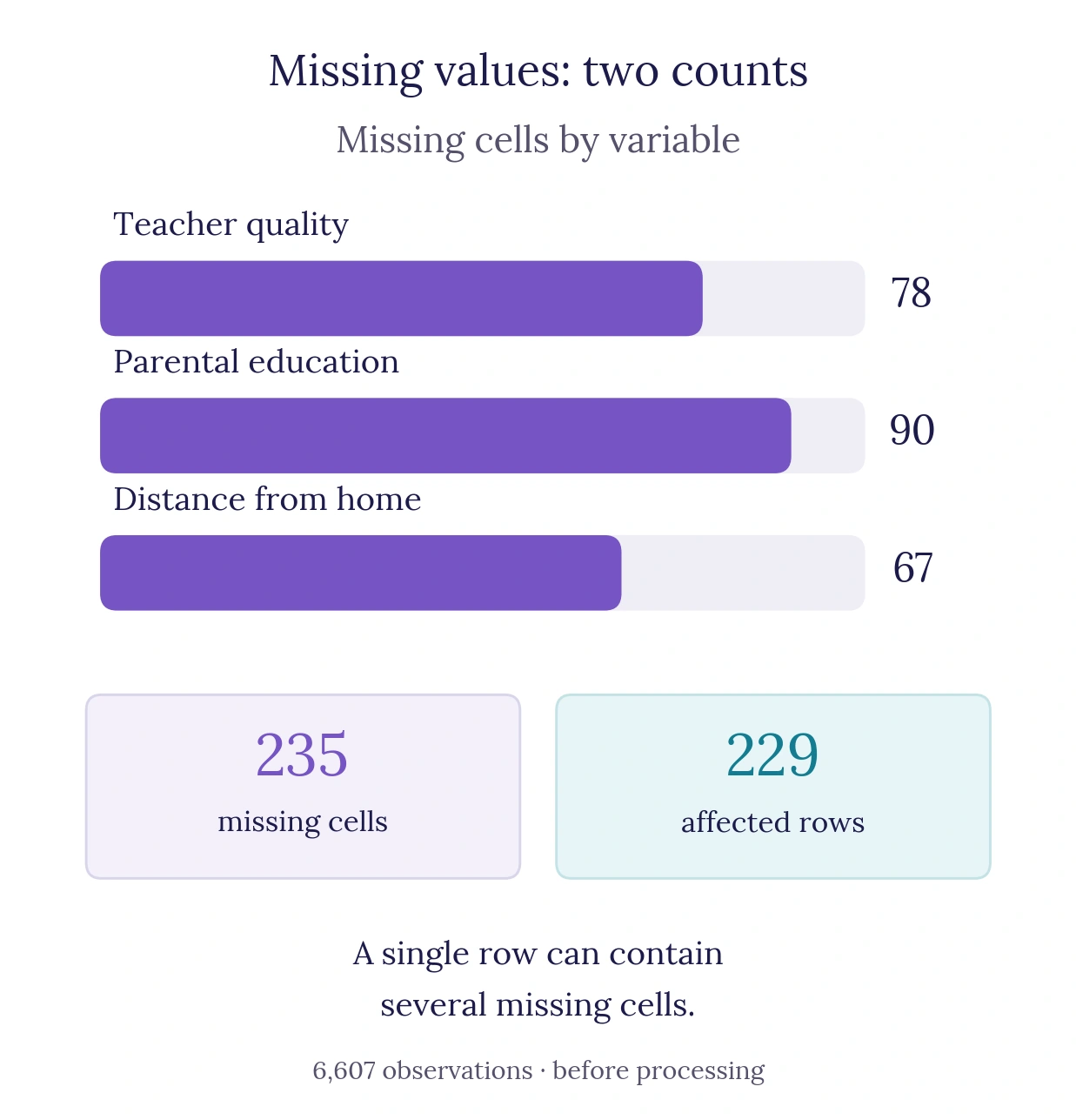
A missing value is information absent for a particular observation and variable. It differs from zero, which can be a valid quantity, and from No, which is a recorded category here. In the version examined, missing cells are distributed as follows:
| Variable | Missing cells | Percentage of rows |
|---|---|---|
Teacher_Quality | 78 | 1.18% |
Parental_Education_Level | 90 | 1.36% |
Distance_from_Home | 67 | 1.01% |
isna() identifies missing values. The first sum() counts them by column; any(axis=1) identifies affected rows. This produces two different totals:
# Distinguish missing cells from affected rows.
missing = df.isna()
by_column = missing.sum()
print(by_column[by_column > 0].to_string())
print("Missing cells:", int(missing.sum().sum()))
print("Affected rows:", int(missing.any(axis=1).sum()))Teacher_Quality 78
Parental_Education_Level 90
Distance_from_Home 67
Missing cells: 235
Affected rows: 229There are 235 missing cells across 229 rows, affecting approximately 3.47% of observations. The numbers differ because one row can contain several missing values. Neither finding, by itself, justifies removing all affected rows or replacing the cells with zero.
An exact duplicate is a row identical to another across the columns compared. Checking all 20 columns in each view finds no exact duplicates. This does not prove that every student appears only once: without a reliable identifier and collection documentation, two different records may still concern the same person.
Also examine unusual values, unexpected categories and contradictions with the definitions. In the regression dataset, one observation has an Exam_Score value of 101. This warrants checking the scoring scale and the source. That number alone cannot tell us whether to keep, correct or exclude it.
duplicated() marks repeated rows in the regression dataset with True; the first occurrence is not marked by default. The following sum() counts the marked rows. Checking the maximum score and values above 100 flags a value to investigate without changing the data:
# Record findings without changing the source.
print("Exact duplicates:", int(df.duplicated().sum()))
print("Maximum score:", df["Exam_Score"].max())
print("Scores above 100:", int(df["Exam_Score"].gt(100).sum()))Exact duplicates: 0
Maximum score: 101
Scores above 100: 16. Write a dataset description and state its limitations
A useful description lets someone else understand what you examined and trace your findings. It identifies the file and version, granularity, task, variables selected for description, summaries and open questions. It separates observed facts from decisions still to be made.
This description does not establish that a model will work in another school. The target population is the set of cases you want to apply the results to. A sound description of the file does not demonstrate that its observations represent that population. Missing dates or school identifiers, for example, limit the checks possible across time and school contexts.
Nor does it establish that increasing study hours would cause a specific rise in exam scores. Describing two variables or observing an association is not enough to establish a causal effect. Other factors, measurement conditions and the way the data were assembled may play a part.
For a predictive project, also distinguish this descriptive inventory from exploration used to choose a model. Set aside test data before using analyses to select inputs, tune transformations or compare algorithms. For example, do not reuse a mean calculated on the full file to fill missing values during model evaluation. Calculate that imputation mean from training data alone. Final evaluation must remain independent of these choices.
Practice: correct a dataset description
You receive this note about the regression dataset:
“The 6,607 rows prove that all the students are different. The 20 columns are model inputs. The 235 missing values concern 235 students: we will replace them with zero. The mean of 19.98 hours shows that each student studies for about 20 hours per week. The score of 101 will be reduced to 100. The file can therefore be used directly to predict scores in every school.”
Identify the claims that the lesson’s findings do not support. Then write a paragraph that retains the useful figures, distinguishes inputs from the target and names at least two checks that are still needed.
Show the explained solution
The row count does not establish people’s identities. The 20 columns include 19 candidate inputs and the Exam_Score target, so they are not all inputs. The 235 missing cells occur across 229 rows, without justifying replacement by zero. The mean summarizes the distribution; it does not describe each student. The value of 101 needs checking against the scoring scale. Finally, use in other schools requires checking the population and intended conditions of use.
One possible revision: “The regression view contains 6,607 observations, 19 potential input variables and the Exam_Score target. Mean study time is 19.98 hours per week, with observed values from 1 to 44 hours. Three columns contain 235 missing cells across 229 rows. No exact duplicates are detected across the 20 columns, but this does not establish that every row represents a different student. Before preparing a model, checks still needed include the scoring scale for a score of 101, input availability and whether the data represent the population for which the model is intended.”
Reproduce a description with Python
Using the regression dataset already loaded, calculate the minimum, median and maximum of Sleep_Hours. Then count observations with no value for Teacher_Quality. Keep the data unchanged and check the unit of each result.
Show the Python solution
Observed sleep duration ranges from 4 to 10 hours per night, with a median of 7 hours. The second output counts 78 missing values in another variable; it is not a duration.
# Describe sleep duration and count missing values in another variable.
print(df["Sleep_Hours"].agg(["min", "median", "max"]).to_string())
print("Missing Teacher_Quality:", int(df["Teacher_Quality"].isna().sum()))min 4.0
median 7.0
max 10.0
Missing Teacher_Quality: 78Common mistakes
- Looking only at the first few rows. A preview helps you read the columns, but may miss rare categories and anomalies. Counts and checks should cover the entire view being described.
- Confusing storage type with statistical meaning. A number can encode a category. Check its definition before calculating a mean or choosing a chart.
- Omitting a percentage’s denominator. State whether it covers all rows or only non-missing values. Those proportions answer different questions.
- Cleaning without recording the finding. Keep the source and document the chosen rule, affected rows and justification. A transformation should be explainable.
- Assuming that an available column is suitable for use. Check its relevance, availability and the data’s terms of use before making it an application input.
Key points and further learning
To describe a dataset before building a model, start with what the rows mean, where the data come from and the question being asked. Define variables and units, separate inputs from the target, then summarize distributions and observed issues. The final description should make unresolved limitations visible.
Sources and further reading
For the Python methods used: reading Excel with pandas, identifying missing values and detecting duplicate rows.
- Student Performance Factors — Kaggle, lainguyn123: the original resource behind the working workbook. The lesson’s counts and summaries were recalculated from the local version.
- Google — Machine Learning Glossary: datasets and machine learning terminology.
- NIST — What is Exploratory Data Analysis?: the exploratory approach to data.
- NIST — Measures of Location: mean, median and sensitivity to extreme values.
- scikit-learn — Data leakage: keeping training and evaluation separate.
